Trace, Laplacian, the Heat equation, divergence theorem
The aim of this article is to help build an intuition for the trace of a matrix, "the sum of the elements on the diagonal" – the basic idea is that the trace is an "average" of some sort, an average of the action of an operator or a quadratic form. We'll make this idea clearer with an example from classical physics: the heat equation.
Consider an n-dimensional space with some temperature distribution T(x⃗,t). We wish to set up a differential equation for this function.
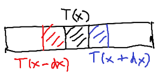
In the case that n = 1, this differential equation is exceedingly easy to write down, considering the difference (T(x+dx)−T(x)) − (T(x)−T(x−dx)) as the double-derivative upon division by dx2. More rigorously, what we're doing here is applying a localised version of the fundamental theorem of calculus. I.e. we're writing down:
$$\begin{align} \lim_{\Delta x \to 0} \frac{1}{\Delta x}(T'(x + \Delta x) - T'(x)) &= \lim_{\Delta x \to 0} \frac{1}{{\Delta x}}\int_x^{\Delta x} {T''(x)dx} \\ & = T''(x) \end{align} $$
More generally, we may consider the n-dimensional case.
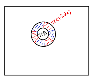
Analogously to before, one may try to look at temperature flows in each direction – here, we have an integral, done on the boundary of an infinitesimal region V (this symbol will also represent the volume of the region):
$$ \frac{{\partial T}}{{\partial t}} = \lim_{V \to 0} \frac{\alpha }{V}\int_{\partial V} {\hat u\,dS \cdot \vec \nabla T} $$
At this point, one may apply the divergence theorem, converting this to:
$$\frac{{\partial T}}{{\partial t}} = \mathop {\lim }\limits_{V \to 0} \frac{\alpha }{V}\int\limits_V {\vec \nabla \cdot \vec \nabla T\;dV} = \alpha{\left| {\vec \nabla } \right|^2}T$$
In this sense, the divergence theorem is analogous to the fundamental theorem of calculus for manifolds with boundaries that are more than one-dimensional (see the bottom of the page for a link to a formalisation/an abstraction based on this analogy). But there are more ways to intuitively understand this. Note how the Laplacian is the trace of the Hessian matrix (note: we use $\vec{\nabla}^2$ to refer to the Hessian and $\left|\vec\nabla\right|^2$ to refer to the Laplacian):
$${\left| {\vec \nabla } \right|^2}T = {\mathop{\rm tr}} \left({\vec{\nabla} ^2}T\right)$$
The trace of a matrix is fundamentally linked to some notion of /averaging/ – the simplest interpretation of this is that it is the mean of the eigenvalues. But more relevant to our situation, it can be shown that the trace of a matrix is the expected value of the quadratic form defined by the matrix on the unit sphere – or on a general sphere S:
$${\mathop{\rm tr}} A = \frac{1}{S}\int_S {\frac{{\Delta {x^T}A\,\Delta x}}{{\Delta {x^T}\Delta x}}\,dS} $$
One may check that taking the limit as Δx → 0, substituting ∇2 for the operator and writing ${\overrightarrow \nabla ^2}f\,d\vec x = \overrightarrow \nabla f$, one gets the original "average of directional derivatives" expression.
Can you interpret the other coefficients of the characteristic polynomial in terms of statistical ideas?
Further reading:
- Using the "infinitesimal region" idea to define divergence, curl and Laplacian rigorously: Khan Academy
- An abstraction based on the "analogy" between FTC, Divergence Theorem, Navier-Stokes Theorem, etc. Stokes' theorem (Wikipedia)